Tidyuesday

library(tidytuesdayR)
library(tidyverse)
library(broom)
library(osmdata)
library(ggthemes)
library(ggforce)
library(gganimate)

sf_trees <- readr::read_csv('https://raw.githubusercontent.com/rfordatascience/tidytuesday/master/data/2020/2020-01-28/sf_trees.csv')
save(sf_trees, file = 'sf_trees.Rdata')

sanfra <- getbb("San francisco")

road.sp1 <- opq(sanfra) %>% 
  add_osm_feature('highway', c('motorway', 'primary', 'secondary', 'tertiary')) %>% 
  osmdata_sf()

road.sp2 <-  opq(sanfra) %>% 
  add_osm_feature('highway') %>%     
  osmdata_sf()

sanfra_list <-  list(road.sp1=road.sp1,
                     road.sp2=road.sp2)

save(sanfra_list,file = "sanfra_list.Rdata")

load("sf_trees.Rdata")
load("sanfra_list.Rdata")

df <-  sf_trees %>% 
  select(c(species,latitude,longitude)) %>% 
  filter(!is.na(latitude)) %>% 
  filter(latitude < 47) %>% 
  mutate(class1 = case_when(str_detect(species,"Brisbane") ~ paste("Brisbane Box\nLophostemon confertus"),
                            str_detect(species,"Sycamore: London Plane") ~ paste("Sycamore London Plane\nPlatanus x hispanica"),
                            str_detect(species,"New Zealand Xmas Tree") ~ paste("New Zealand Christmas Tree\nMetrosideros excelsa"),
                            str_detect(species,"Hybrid Strawberry Tree") ~ paste("Hybrid Strawberry Tree\nArbutus 'Marina'"),
                            str_detect(species,"Maytenus") ~ paste("Mayten\nMaytenus boaria"),
                            str_detect(species,"Corymbia ficifolia") ~ paste("Red Flowering Gum\nCorymbia ficifolia"),
                            str_detect(species,"runus cerasifera :: Cherry Plum") ~ paste("Cherry Plum\nPrunus cerasifera"),
                           TRUE~"Others"),
         class2 = case_when(str_detect(species,"Brisbane") ~ "2",
                            str_detect(species,"Sycamore: London Plane") ~ "3",
                            str_detect(species,"New Zealand Xmas Tree") ~ "4",
                            str_detect(species,"Hybrid Strawberry Tree") ~ "5",
                            str_detect(species,"Maytenus") ~ "6",
                            str_detect(species,"Corymbia ficifolia") ~ "7",
                            str_detect(species,"runus cerasifera :: Cherry Plum") ~ "8",
                           TRUE~"1")) %>% 
  group_by(class1) %>% 
  add_tally()
  

g <- ggplot()+
  geom_sf(data = sanfra_list$road.sp1$osm_lines, col = 'white', size = .2) +
  geom_sf(data = sanfra_list$road.sp2$osm_lines, col = 'white', size = .05) +
  geom_sf(data = sanfra_list$road.sp1$osm_lines, col = alpha('grey60',.2), size = 1.3) +
  geom_sf(data = sanfra_list$road.sp2$osm_lines, col = alpha('grey60',.2), size = .4) +
  geom_point(data = df %>% filter(class2 == "1"),aes(x=longitude , y=latitude, color=class2),size=1.5, alpha=.5) +
  geom_circle(aes(x0 = -122.323, y0 = 37.78, r = .007), color="#2E2926" ,fill="#2E2926")+
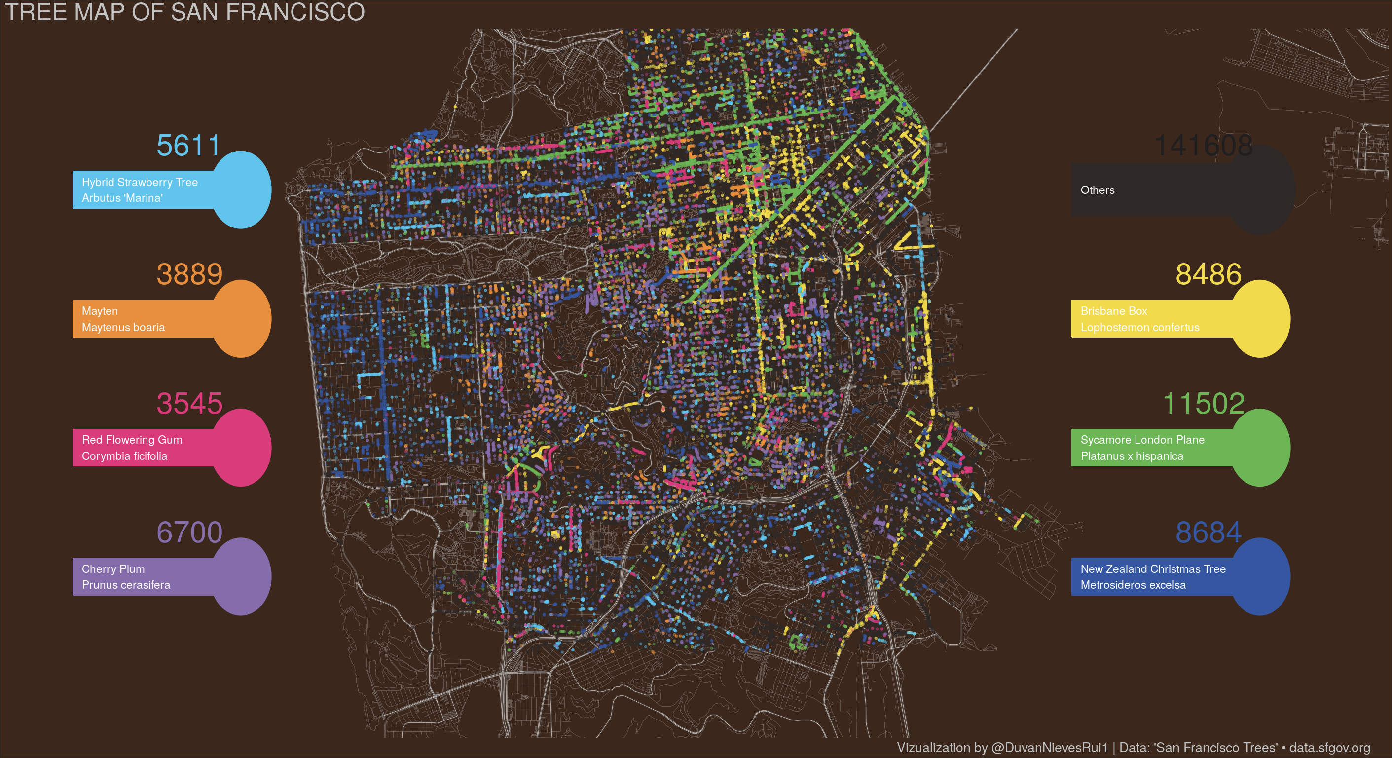
  geom_label(aes(x=-122.36,y=37.78,label=paste("\nOthers                                         \n")),show.legend = F,fill="#2E2926",size=6, color="white",label.size = 0,
             hjust=0, label.padding = unit ( .7, "lines" ))+
  annotate(geom = 'text',x=-122.334,y=37.787, label ="141608" , color="#201E1F" ,size=16)+
  geom_point(data = df %>% filter(class2 == "2"),aes(x=longitude , y=latitude, color=class2),size=1.5, alpha=.4) +
  geom_circle(aes(x0 = -122.323, y0 = 37.76, r = .006), color="#F1DA4C" ,fill="#F1DA4C")+
  geom_label(aes(x=-122.36,y=37.76,label=paste("Brisbane Box\nLophostemon confertus            ")),show.legend = F,fill="#F1DA4C",size=6, color="white",
             label.size = 0, hjust=0, label.padding = unit ( .7, "lines" ))+
  annotate(geom = 'text',x=-122.333,y=37.767, label ="8486" , color="#F1DA4C" ,size=16)+
  geom_point(data = df %>% filter(class2 == "3"),aes(x=longitude , y=latitude, color=class2),size=1.5, alpha=.4) +
  geom_circle(aes(x0 = -122.323, y0 = 37.74, r = .006), color="#6CB655" ,fill="#6CB655")+
  geom_label(aes(x=-122.36,y=37.74,label=paste("Sycamore London Plane           \nPlatanus x hispanica")),show.legend = F,fill="#6CB655",size=6, color="white",
             label.size = 0, hjust=0, label.padding = unit ( .7, "lines" ))+
  annotate(geom = 'text',x=-122.334,y=37.747, label ="11502" , color="#6CB655" ,size=16)+
  geom_point(data = df %>% filter(class2 == "4"),aes(x=longitude , y=latitude, color=class2),size=1.5, alpha=.4) +
  geom_circle(aes(x0 = -122.323, y0 = 37.72, r = .006), color="#3557A1" ,fill="#3557A1")+
  geom_label(aes(x=-122.36,y=37.72,label=paste("New Zealand Christmas Tree   \nMetrosideros excelsa")),show.legend = F,fill="#3557A1",size=6, color="white",
             label.size = 0, hjust=0, label.padding = unit ( .7, "lines" ))+
  annotate(geom = 'text',x=-122.333,y=37.727, label ="8684" , color="#3557A1" ,size=16)+
  geom_point(data = df %>% filter(class2 == "5"),aes(x=longitude , y=latitude, color=class2),size=1.5, alpha=.4) +
  geom_circle(aes(x0 = -122.523, y0 = 37.78, r = .006), color="#61C4ED" ,fill="#61C4ED")+
  geom_label(aes(x=-122.556,y=37.78,label=paste("Hybrid Strawberry Tree     \nArbutus 'Marina'")),show.legend = F,fill="#61C4ED",size=6, color="white",label.size = 0,
             hjust=0, label.padding = unit ( .7, "lines" ))+
  annotate(geom = 'text',x=-122.533,y=37.787, label ="5611" , color="#61C4ED" ,size=16)+
  geom_point(data = df %>% filter(class2 == "6"),aes(x=longitude , y=latitude, color=class2),size=1.5, alpha=.4) +
  geom_circle(aes(x0 = -122.523, y0 = 37.76, r = .006), color="#E88F3D" ,fill="#E88F3D")+
  geom_label(aes(x=-122.556,y=37.76,label=paste("Mayten\nMaytenus boaria                  ")),show.legend = F,fill="#E88F3D",size=6, color="white",
             label.size = 0, hjust=0, label.padding = unit ( .7, "lines" ))+
  annotate(geom = 'text',x=-122.533,y=37.767, label ="3889" , color="#E88F3D" ,size=16)+
  geom_point(data = df %>% filter(class2 == "7"),aes(x=longitude , y=latitude, color=class2),size=1.5, alpha=.4) +
  geom_circle(aes(x0 = -122.523, y0 = 37.74, r = .006), color="#DA3B7B" ,fill="#DA3B7B")+
  geom_label(aes(x=-122.556,y=37.74,label=paste("Red Flowering Gum\nCorymbia ficifolia                 ")),show.legend = F,fill="#DA3B7B",size=6, color="white",
             label.size = 0, hjust=0, label.padding = unit ( .7, "lines" ))+
  annotate(geom = 'text',x=-122.533,y=37.747, label ="3545" , color="#DA3B7B" ,size=16)+
  geom_point(data = df %>% filter(class2 == "8"),aes(x=longitude , y=latitude, color=class2),size=1.5, alpha=.4) +
  geom_circle(aes(x0 = -122.523, y0 = 37.72, r = .006), color="#856DAB" ,fill="#856DAB")+
  geom_label(aes(x=-122.556,y=37.72,label=paste("Cherry Plum\nPrunus cerasifera               ")),show.legend = F,fill="#856DAB",size=6, color="white",
             label.size = 0, hjust=0, label.padding = unit ( .7, "lines" ))+
  annotate(geom = 'text',x=-122.533,y=37.727, label ="6700" , color="#856DAB" ,size=16)+
  scale_color_manual(values = c("1" ="#2E2926","2"="#F1DA4C","3"="#6CB655","4"="#3557A1","5"="#61C4ED","6"="#E88F3D","7"="#DA3B7B","8"="#856DAB")) +
  coord_sf(xlim = c(-122.557,-122.31), ylim = c(37.7,37.8), expand = T)+
  labs(title = "TREE MAP OF SAN FRANCISCO",
       caption = "Vizualization by @DuvanNievesRui1 | Data: 'San Francisco Trees' • data.sfgov.org") +
  theme_map()+
  theme(legend.position = "none",
        axis.title =  element_blank(),
        axis.ticks =  element_blank(),
        axis.line = element_blank(),
        axis.text.x = element_blank(),
        axis.text.y = element_blank(),
        panel.background = element_rect(fill="#3B271C",color = "#3B271C"),
        plot.background = element_rect(fill="#3B271C"),
        panel.spacing = unit(.5, "lines"),
        plot.title = element_text(size=36, color="grey76",hjust = 0),
        plot.caption = element_text(size = 20,color = "grey76", hjust = .98))

g

g1 <- g +  transition_layers(layer_length = 1,transition_length = 1) +
  shadow_mark()+  enter_grow()+
  exit_fade() + exit_shrink()


animate(g1, renderer = gifski_renderer(),height = 500, width = 1000,fps = 10)